

The AirScope UI App consists of 3 main sections:
1) The SCOPE DISPLAY where the traces are drawn.
2) The CONTROLS PANEL which contains the major UI functions.
3) The BACK PANEL which contains less used functions and settings.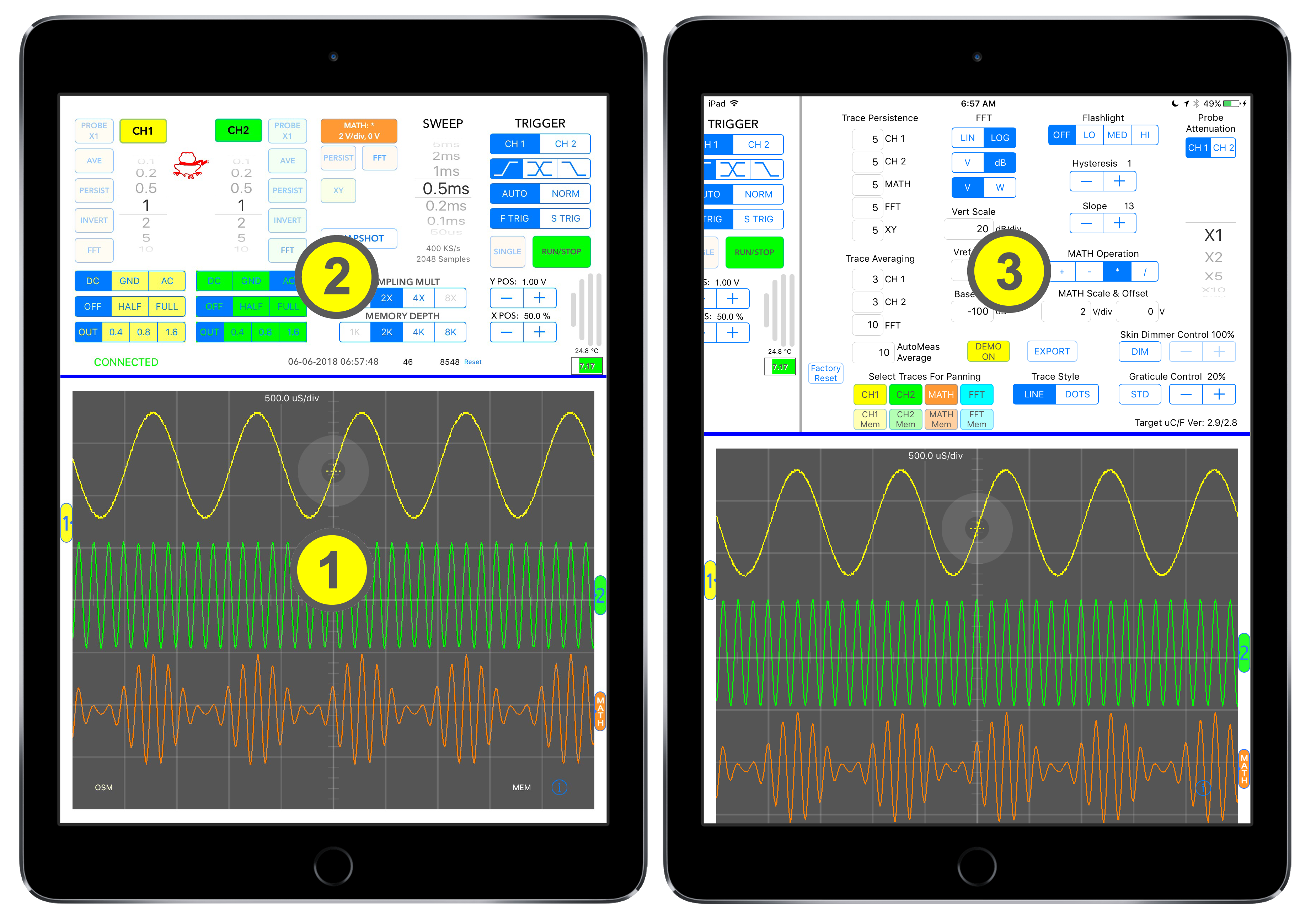
To access the back panel, start at the finger grip area on the right side and swipe the controls panel to the left. The AirScope will still operate in the state and the Run/Stop button is still available. Similarly slide controls to the right to close the back panel.
SCOPE DISPLAY
Basic: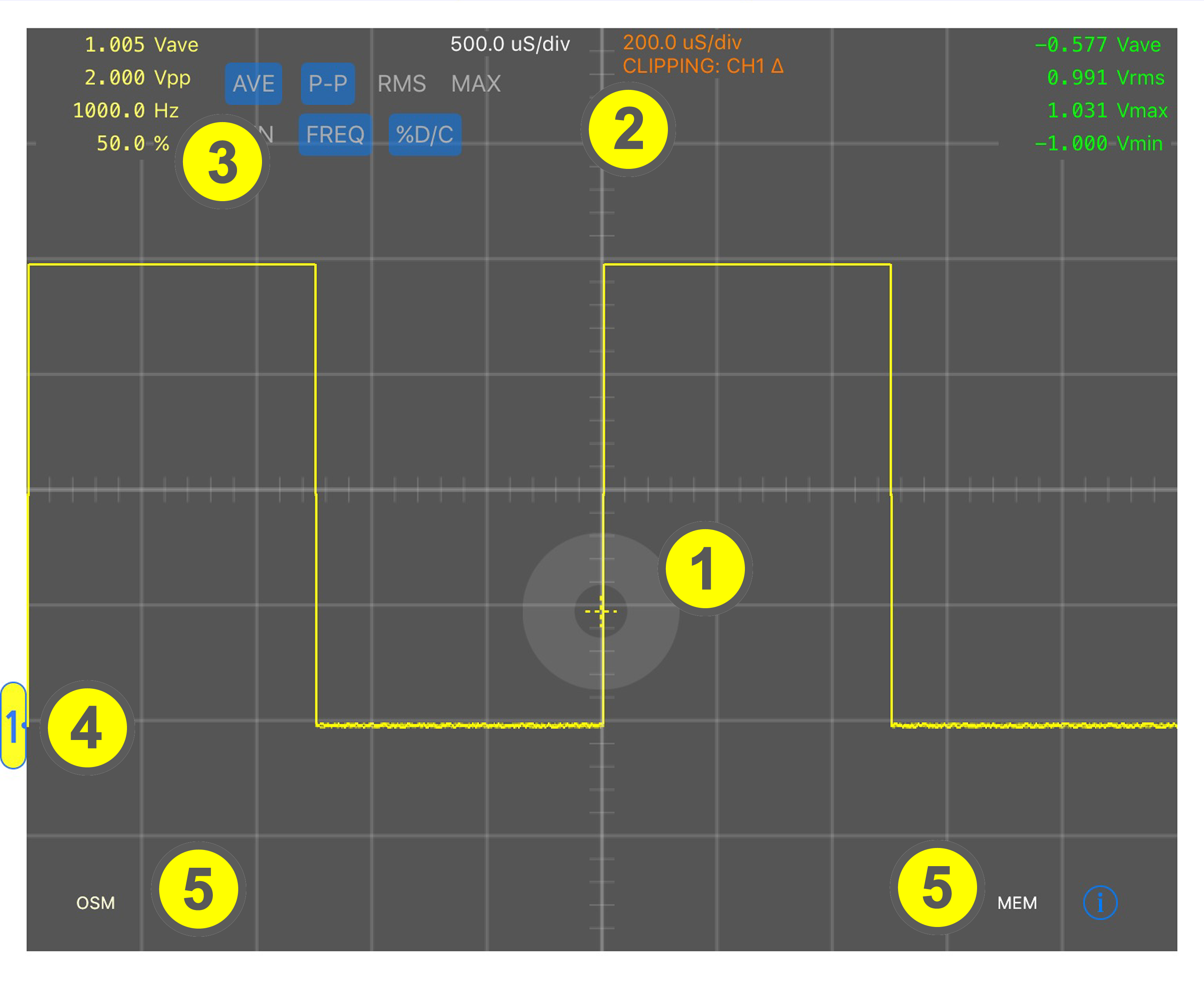
This image shows a typical active display elements.
1) This is the drag & drop trigger cursor. Touch and hold anywhere on the doughnut shaped handle and it will illuminate and become active. Drag it to the desired trigger point and release.
2) This area show a number of operational indicators. The white colored sweep rate value is always visible. The top orange indicator shows the equivalent sweep rate because this trace has been expanded horizontally with a pinch/expand gesture. Also, although it is hard to tell, the top of this trace is clipped because the signal exceeded input range. The Clipping indicator indicates which channel and which side of the signal is clipping. Trigger cursor off screen indicators appear if the triggering trace is positioned vertically so that the trigger cursor goes off screen. The indicator helps locate the trigger cursor. This only applies to vertical trace positioning.
3) Auto measurements can be shown with channel 1 measurements in the upper left and channel 2 in the upper right. A single tap in either corner will cause a panel of selection buttons to fly out. Available measurements are; Vave, Vpp, Vrms, Vmax, Vmin, Frequency and Duty Cycle. Up to 4 measurements can be displayed for each channel. The order in which the buttons are selected determines the display order of the measurements. Tapping the corner area again hides the buttons.
4) Various positioning handles are locate on the vertical edges of the display depending on what traces are turned on. Also various measurement cursor sliders may be shown in the top and bottom white spaces depending on what analysis tools are selected.
5) On-Screen measurement tools are available for both the time domain (OSM) and frequency domain (FFT) displays as well as a trace memory control (MEM) panel and a help/info feature (i). Tapping each will deploy and retract the respective functional panel. The FFT button is only shown if the FFT function is operating.
Mixed Mode Operation:
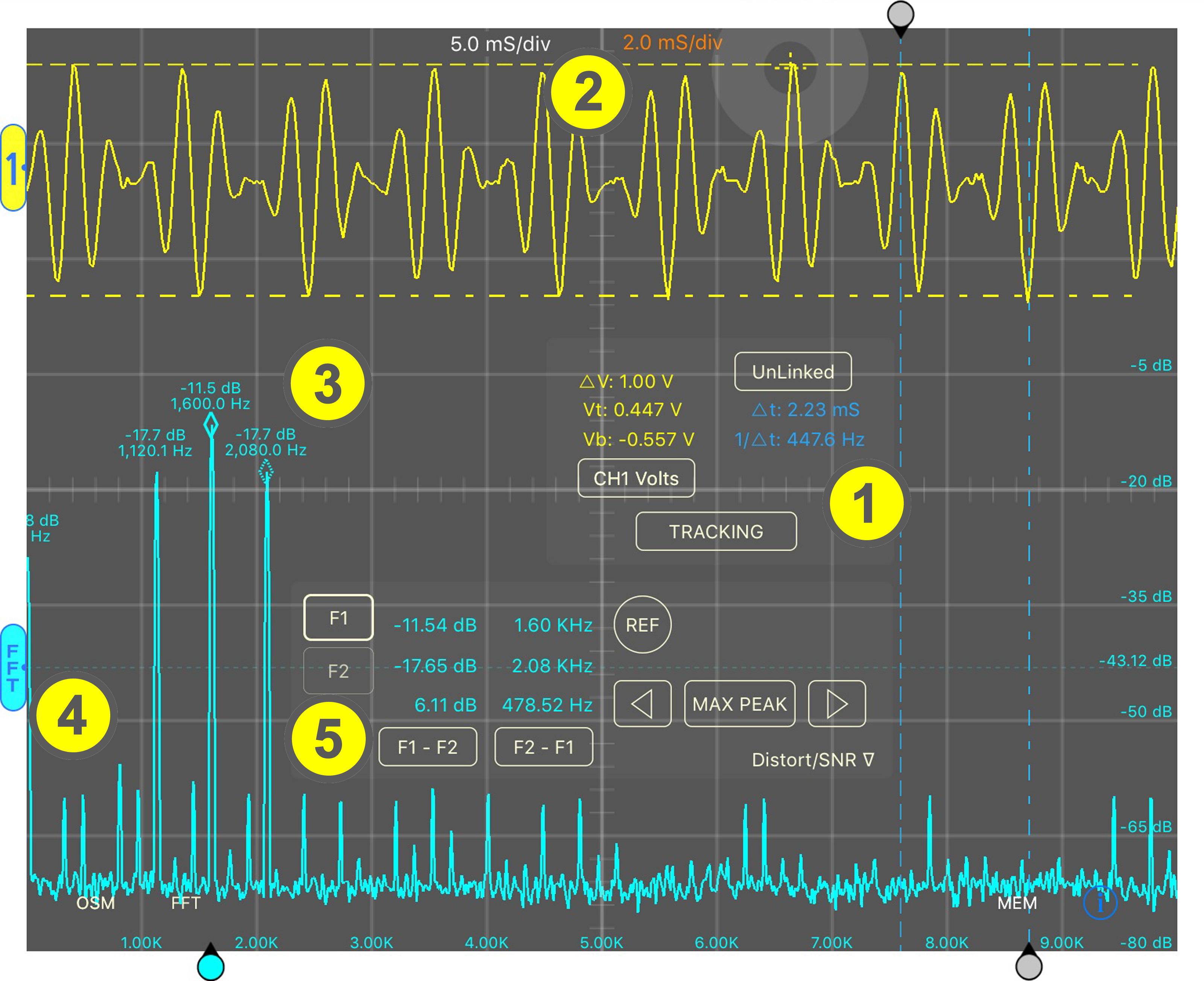 Here’s a mixed mode display showing the time domain trace of a 1.6KHz carrier modulated by 480Hz and it’s spectrum.
1) The time domain On Screen Measurement tool is deployed and is measuring the peak to peak signal level. The tool is in Tracking mode so the horizontal voltage cursors will track the waveform as the vertical cursors are moved. The gray sliders at the top and bottom of the display control the cursor positions and can be nudged one data point at a time for fine positioning by tapping on either side of the slider. In Manual mode the horizontal cursors would have their own sliders and would act independently of the vertical ones. The measurements panel can be dragged anywhere in the scope display.
2) The time domain trace has been expanded with a pinch/expand action to make the waveform’s shape more visible. The expanded trace is noted by the orange equivalent sweep rate indicator to the right of the standard sweep rate value in white. The indicator show the time/div that should be used when evaluating the expanded trace using the graticule divisions.
3) The FFT peak labels are automatically created and any peaks above the FFT reference line (4) are displayed. Peak labels can set to display either dB or millivolts when using a log scale. A linear scale can also be selected.
4) The FFT Reference Line is used to control the display of the magnitude and frequency values of spectrum peaks as well as being a basic measuring tool. Peak data will be displayed for any peaks that are above the FFT Reference Line. The far right end of the dashed reference line shows its current level.
5) The FFT On Screen Measurement tool is showing only the Markers tool (Distortion/Noise tool is rolled up). Its markers are positioned on the carrier and upper sideband peaks and the tool’s readouts show the peaks’ individual magnitudes, frequencies and and the difference between them. Markers can be positioned manually by sliding the bottom pointer or by using the Max Peak and next peak left/right buttons. The Markers slider can be nudged one data point at a time by tapping on either side of the pointer for exact positioning. The measurements panel can be dragged anywhere in the scope display.
The FFT trace can be panned independently from the time domain trace, it can also be expanded and compressed using a pinch gesture. The bottom graticule space is sensitive to these gestures. Sliding a finger horizontally within the bottom graticule division will pan the FFT display and likewise for pinch gesturing. The pinch action must be horizontal to work. Gesturing above the bottom graticule division will cause the time trace to be affected. A single tap anywhere within the Scope Display will recenter all traces and reset any expansion or compression applied of the traces.
FFT Analysis Tools
A set of FFT analysis tools are available to explore the FFT spectrum trace and allow distortion and noise measurements. The tool is available when the FFT function is active on any trace. The FFT button at the bottom left of the scope display deploys or retracts the tool.
FFT Markers Analysis Tool:
The Markers Analysis tool allows frequency and amplitude measurements to be taken off of the FFT trace either by manually moving the marker cursor or by navigating from peak to peak. Two markers allow comparative measurements between marker locations to be made. The F1 marker amplitude can be set as the 0 dB level for making relative amplitude measurements. Available functionality changes as the amplitude units are set to dB or volts, and when the amplitude scaling is switched between log and linear. The lightweight measurements panel can be dragged anywhere within the scope display. Here the Distortion/SNR panel section has been rolled up.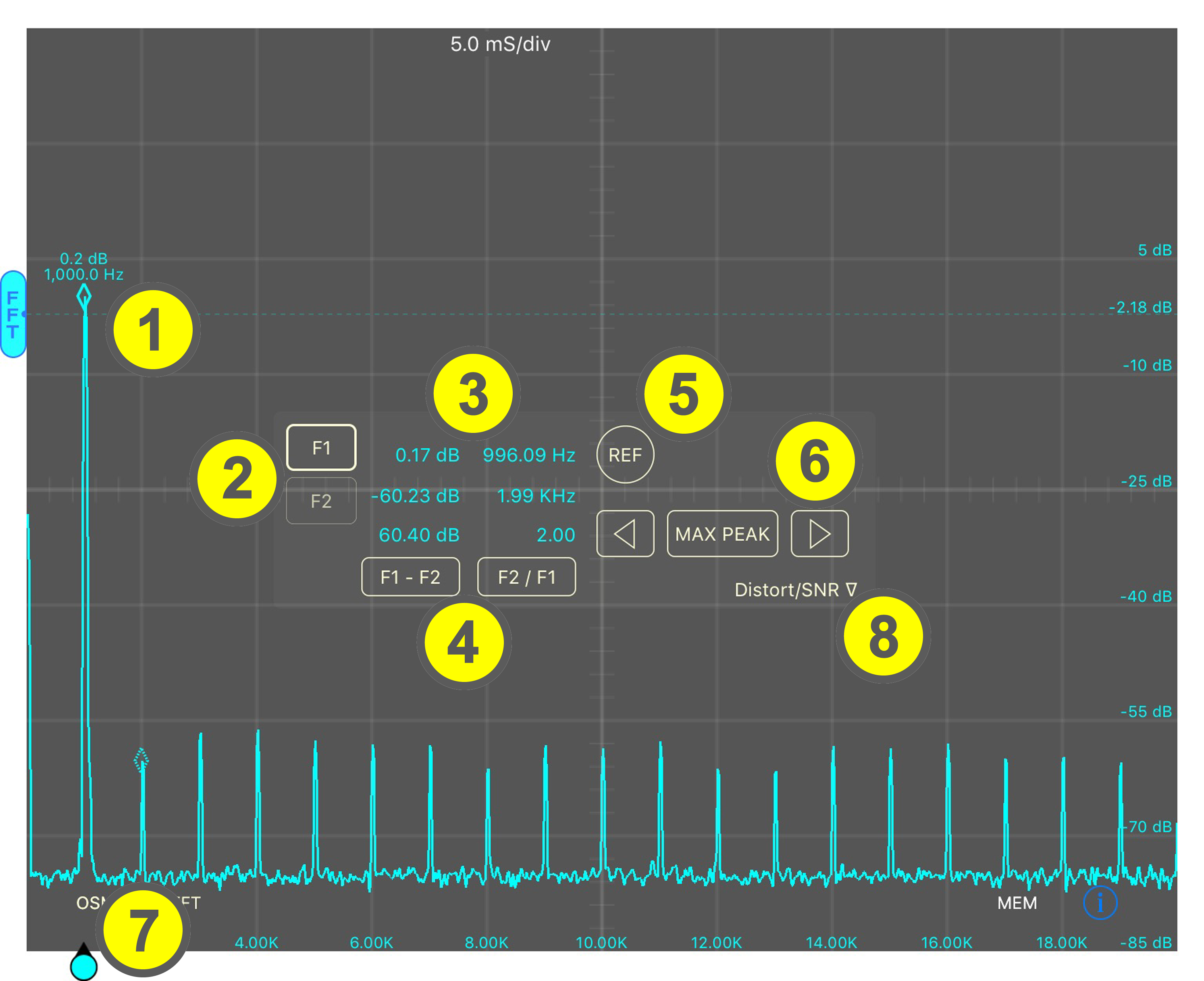
1) The diamond shaped markers indicate the measurement point. The active marker, the one that will be moved, is solid and the inactive one is dashed. Although it is not a function of the Markers tool, the frequency and amplitude data for spectral peaks is displayed when the FFT Ref line is positioned below the peak.
2) The F1 and F2 buttons selected the active marker. The buttons are interlocked so only one marker can be active at a time.
3) There is an amplitude and frequency readout for each of the markers. The units used for amplitude are determined by the FFT settings on the back panel.
4) The readout function buttons either subtract or divide the values in the F1 and F2 amplitude and frequency readouts with the result displayed immediately above the button. The buttons cycle through 4 functions F1-F2, F2-F1, F1/F2 and F2/F1.
5) The REF button will set the current amplitude value in F1 as the 0dB level and changes the value in F2 to reflect the new reference level. When the REF function is active the button’s label is red. This function is only available when the readout units are dB.
6) The marker can be moved from peak to peak but using the peak navigation buttons. The MAX PEAK button finds the largest peak in the spectrum. The arrow buttons move the marker one peak to the right or left.
7) The markers can be moved manually using the slider at the bottom of the display. In order to allow for fine positioning of the marker, the slider can be nudged one data point at a time by tapping to the right or left of the slider icon.
8) The Distortion/SNR panel can be deployed using the associated button. FFT Markers panel can then be rolled up when not needed to declutter the scope display area.
Distortion/SNR Analysis Tool:
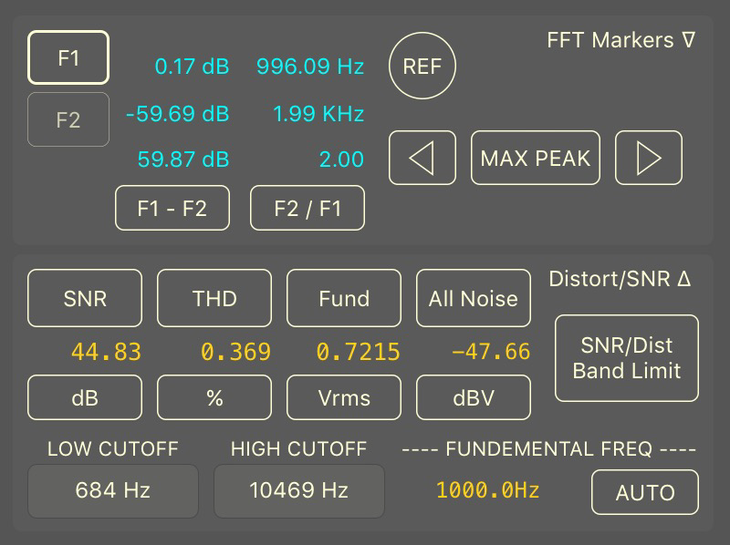
This tool is part of the FFT On Screen Measurement tools and provides 4 independent measurement readouts of various noise and distortion related functions. The bandwidth of the measurement spectrum can be limited both on the low and high sides, or set to the full measurement bandwidth. The lightweight measurements panel can be dragged anywhere within the scope display. Here the Markers panel section has been rolled up.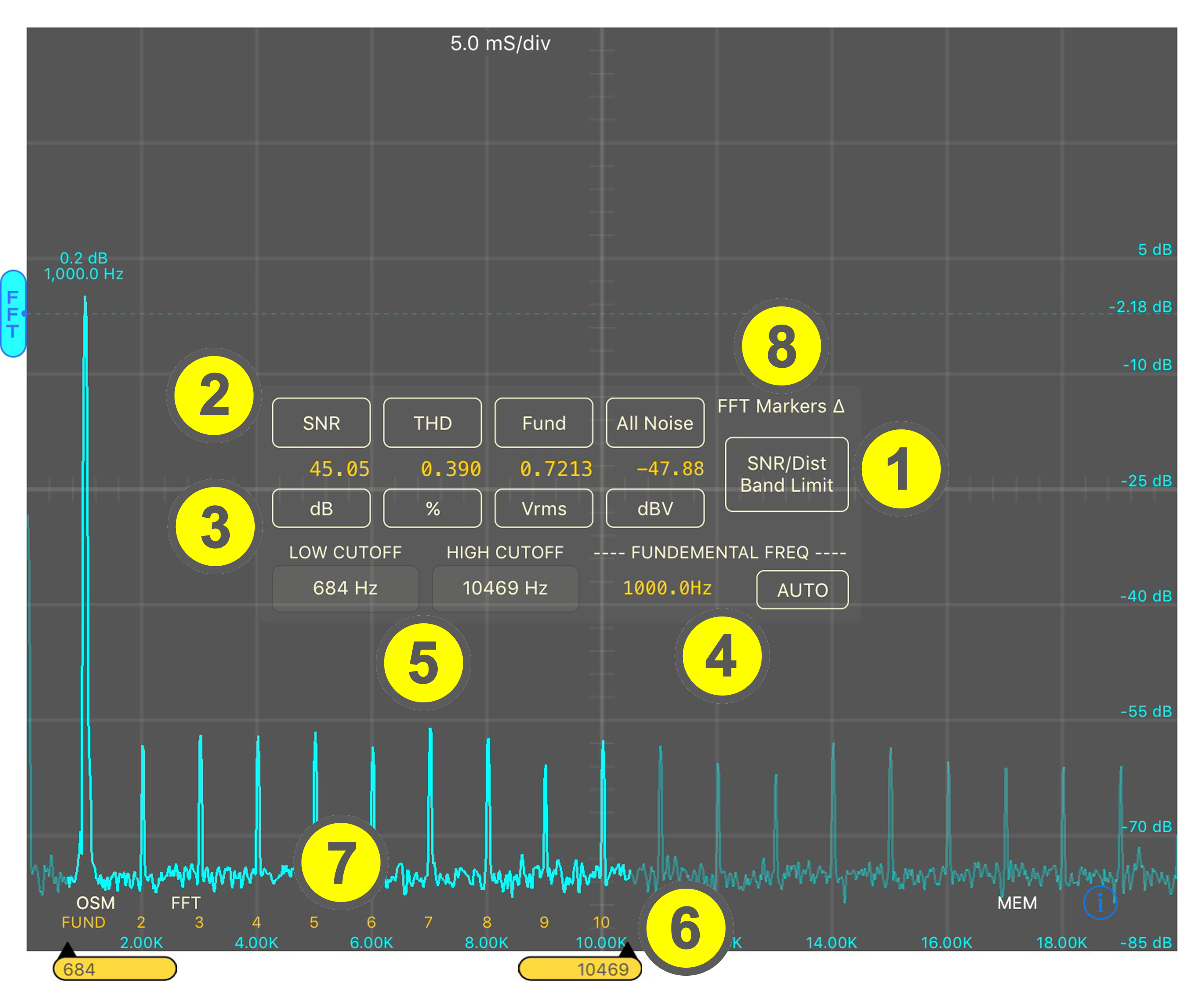
1) The Analysis Mode button allows either full bandwidth of limited bandwidth operation. An Off selection is also available. Since the tool uses a significant amount of processing power, setting the mode to Off when not in use is recommended.
2) The Measurement Selection buttons determine the contents of the readouts. The buttons cycle through the following selections: Off, SNR, SINAD, THD, THD+N, Fundamental, Harmonic Peaks, Noise Peaks, Random Noise and All Noise. The first 4 measurements are standard measurements, the Fundamental selection displays voltage or frequency of the fundamental frequency used for distortion and SNR related measurements. Harmonic Peaks measures the RMS sum of all the peaks harmonically related to the fundamental within the measurement bandwidth. Noise Peaks measures the RMS sum of all spectral peaks within the measurement bandwidth that are not harmonically related to the fundamental. Random Noise measures the RMS value of the non-correlated noise in the FFT. All Noise provides a single value for the sum of all noise types (Harmonic Peaks value is not included here since it is not noise related).
3) The Units Selections buttons allows measurements to be represent in various units. The unit selections vary according to the measurement selected but can include: Vrms, dBV, %, dB, Ratio and Hz.
4) The Fundamental Frequency area provides a mode button, readout or entry field to provide the analysis tool with the proper signal to use as the basis of the SNR and distortion related measurements. The mode button cycles through Off, Manual and Auto. In Auto mode the largest peak within the measurement bandwidth is used as the fundamental. In Manual mode, the value entered in the text field will be used as the fundamental frequency. Off mode will stop the analysis of measurements that require a fundamental frequency value.
5) The Low and High Cutoff text fields allow the band limits to be entered. Entered values will be converted to the closest value that conforms to the resolution of the FFT bins.
6) The measurement bandwidth can also be adjusted by using the cutoff sliders at the bottom of the scope display. The cutoff frequency value is shown in the slider as well as in the Cutoff text fields (5).
7) Harmonic Labels are displayed just above the X-Axis frequency. These labels are displayed when the Distortion/Noise Analysis tool is operating with a valid fundamental frequency. The label FUND indicated the fundamental peak with all other harmonic peaks indicating their harmonic multiple.
8) The Distortion/SNR tool can be rolled up to declutter the display when not needed, however, at least one of the FFT measurement tools must always be displayed. So the FFT Markers tool panel can be deployed using the provided button. Once that is available the Distortion/Noise tool can then be rolled up
OSM Time Trace Tool:
Measurements can be taken off of the time domain traces using the OSM tool. In Manual mode positioning of both horizontal and vertical measurement cursors is accomplished using sliders. In Tracking mode only the vertical (time) cursors are movable with the horizontal (voltage) cursors tracking the waveform voltage data.
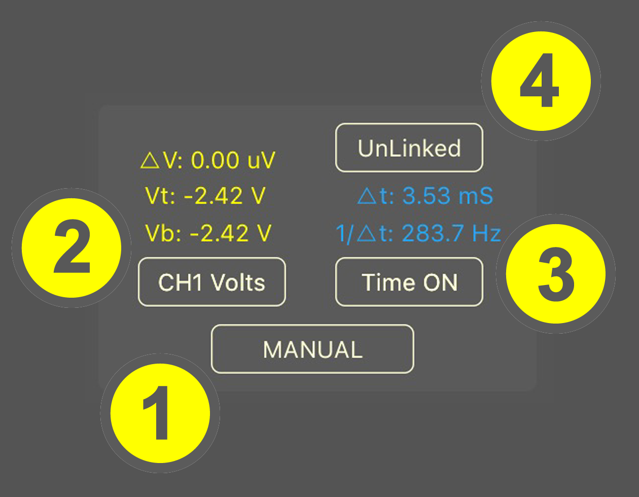 1) Mode button toggles between Manual and Tracking modes.
2) The voltage data area shows the level of each cursor and the difference between them. A button selects which channel is being measured and provides an off setting in Manual mode. This eliminates the horizontal cursors if not needed to decultter the scope display.
3) The time cursors can be turned off in manual mode using this button. This can help to declutter the scope display. In Tracking mode the button is not available.
4) The time cursors can be linked so that they maintain the same spacing while they are moved across the screen. This button is not available when the time cursors are turned off.
Here is an example of the scope display with the OSM tool deployed. The OSM panel can be dragged to any convenient location within the scope display.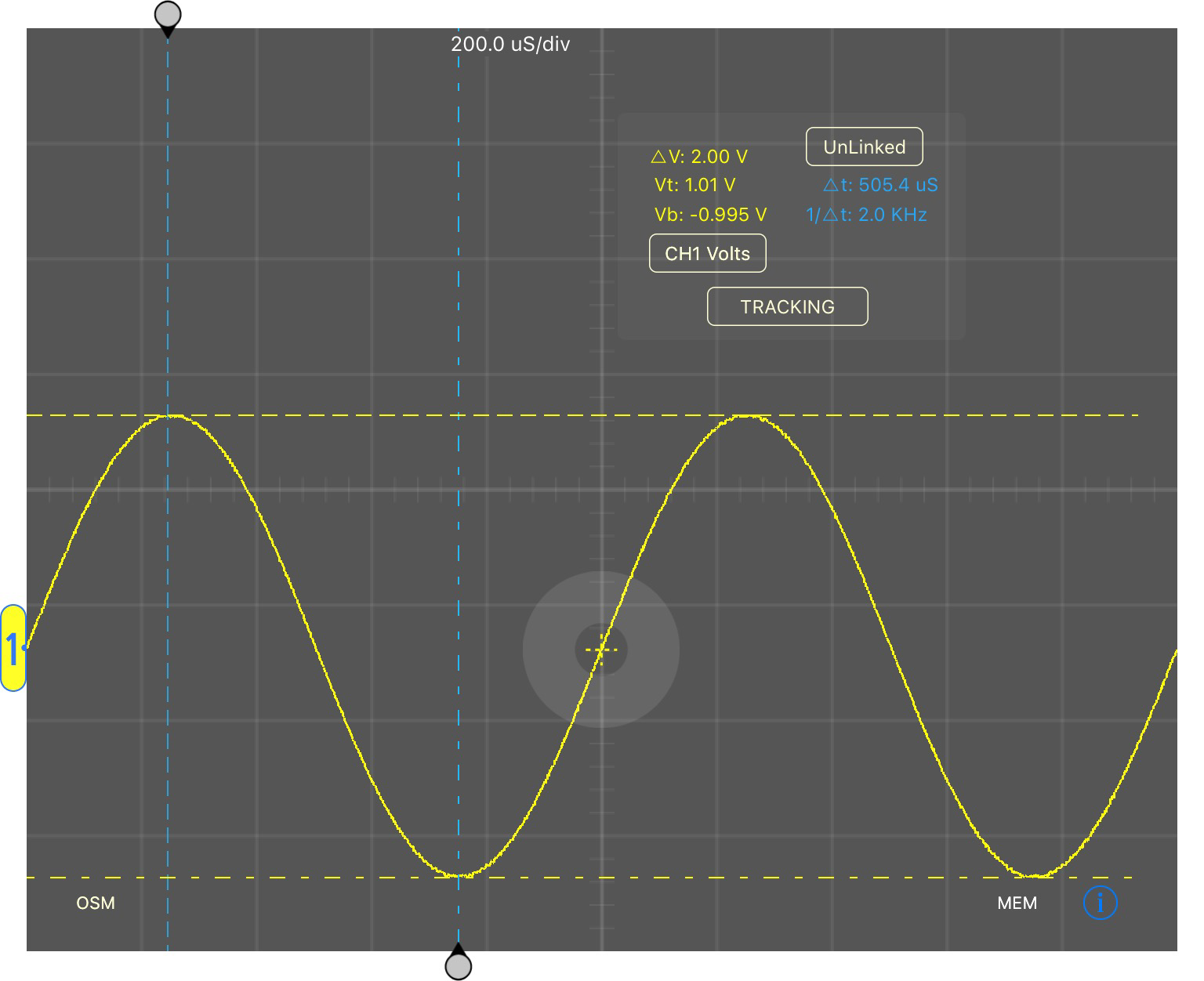
The OSM tool is in tracking mode so the horizontal voltage cursors will track the waveform as the vertical time cursors are moved. If the OSM was in Manual mode, there would be sliders available for each voltage cursor. These cursors can be nudged by tapping on either side of the icon to allow for fine positioning of the cursors.
The gray pointers at the top and bottom of the display are the time cursor sliders. These can be nudged one data point at a time by tapping on either side of the icon.
Scrubber View:
The length of the trace that can be shown in the scope display is fixed by the Sweep Rate (time/div) and then number of graticule divisions. It is possible to configure the AirScope to capture a trace that is longer in time than what can be viewed. When this condition exists the Scrubber View is deployed.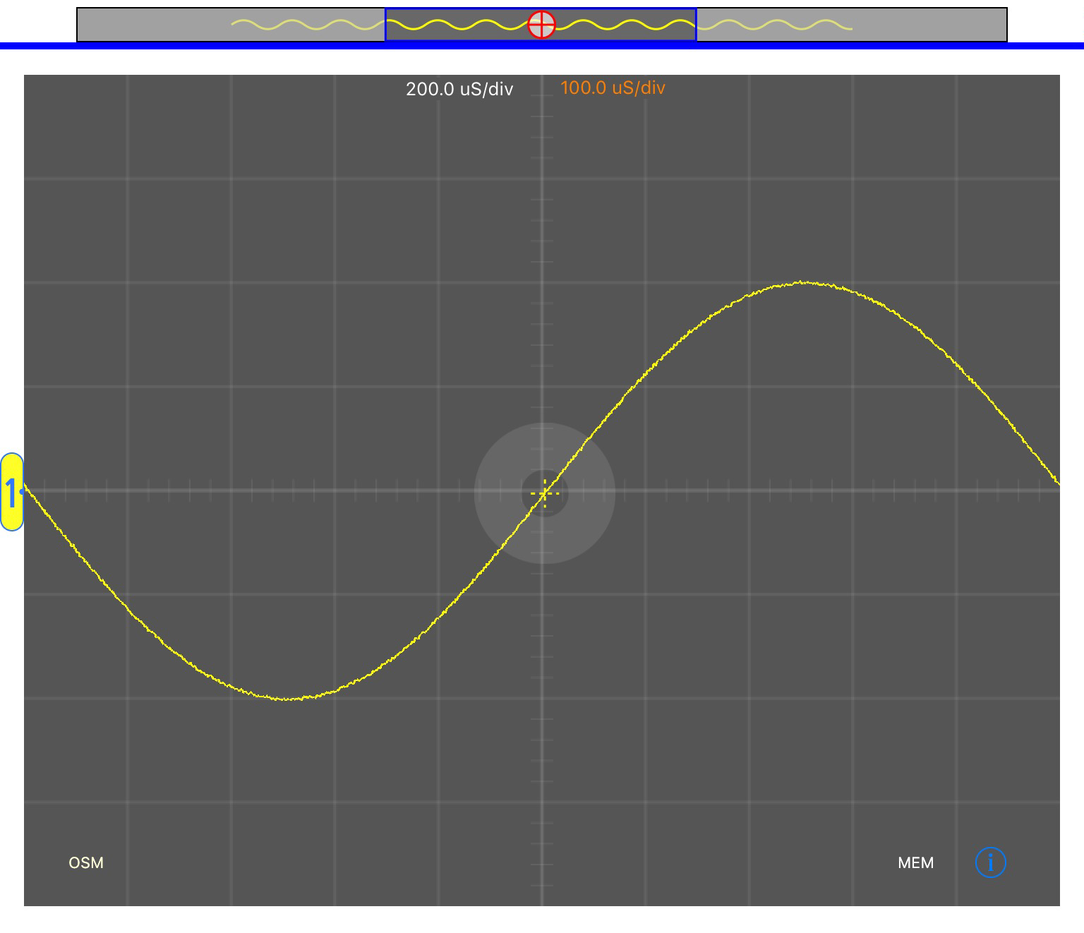
In this image the trace has been expanded using a pinch/expand action so it now is twice as long as what can be shown. The Scrubber View shows where on the entire captured trace the visible display is located. The mock trace in yellow represents the entire trace with the darkened, blue outlined, area representing the visible display. The red trigger icon represents the position of the trigger on the entire trace.
As the scope display is panned, the visible display icon will move to reflect the new postion. The Scrubber View also allows for fast panning along the trace by dragging the visible display icon. The trigger icon can also be dragged to quickly reposition the trigger’s horizontal position. To grab the trigger icon the visible display must first be moved out of the way. If the visible display icon become too small to grab, a dotted line rectangle will indicate the touch target area to grab the icon.
The Scrubber View works with both the time domain and the FFT traces. If both traces cause the Scrubber View to deploy, a button appears to the left of the view to select which trace will be affected by the Scrubber actions.
Trace Memories:
A lightweight, re-positional, fly out panel controlling the storage and viewing options for the different traces is available by tapping the MEM button in the lower right corner of the scope display area.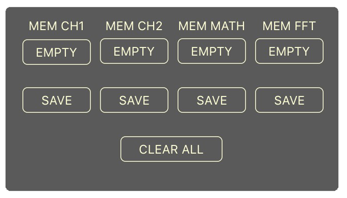
In order to be saved, Math and FFT functions must be active. A button for each trace allows the saved data to be shown or hidden. A Clear All button is provided to empty all trace memories of data. As each stored trace is shown on the scope display an associated vertical positioning handle appears. Trace memories can be locked from panning horizontally.
Graticule:
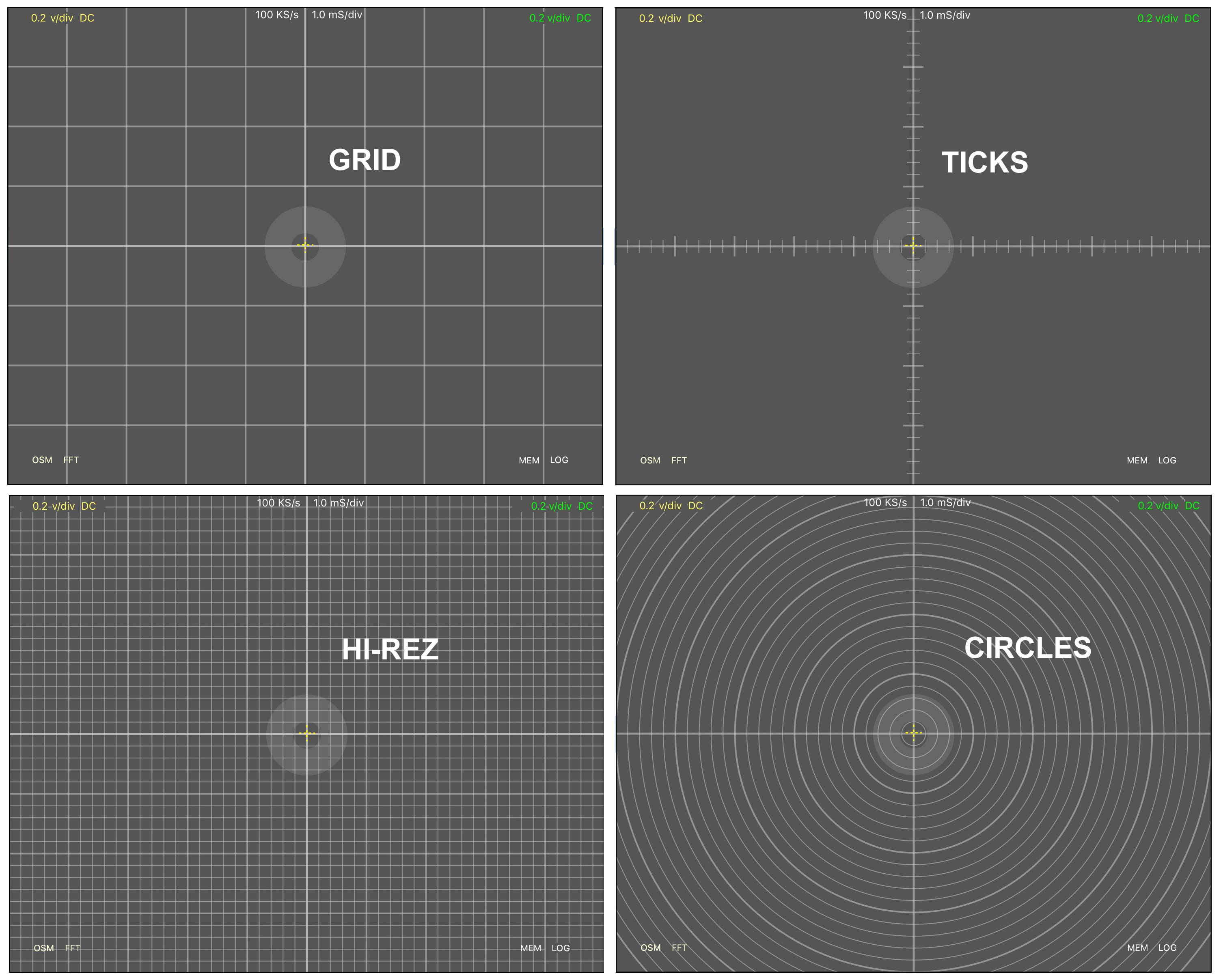
5 Types of graticule are provided to assist in evaluating trace data (STD style is shown in the Basic image at the start of this section).
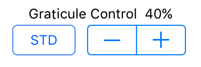 These controls allow graticule selection and intensity control. The graticule sits on top of the traces.
CONTROLS PANEL
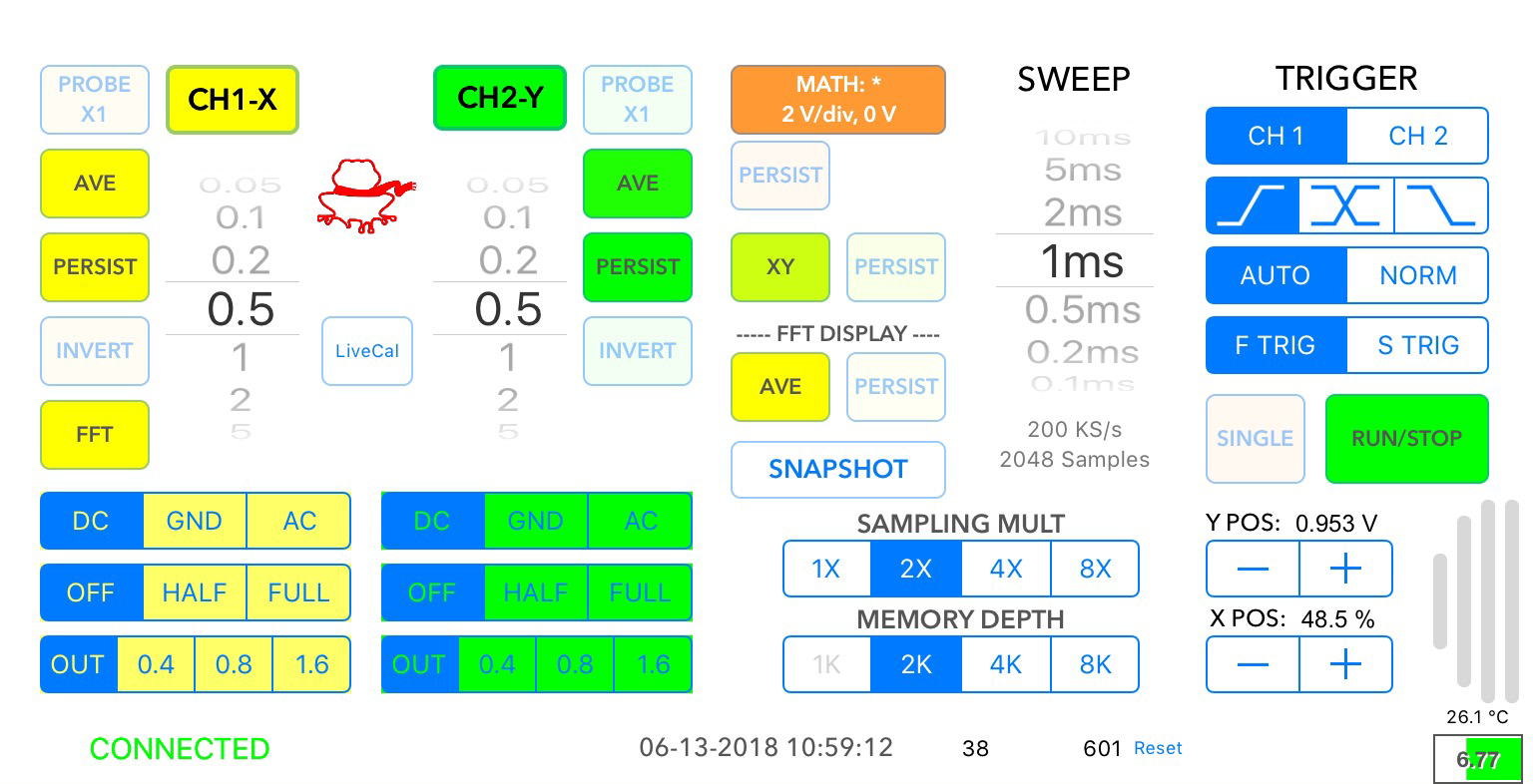
Input Controls
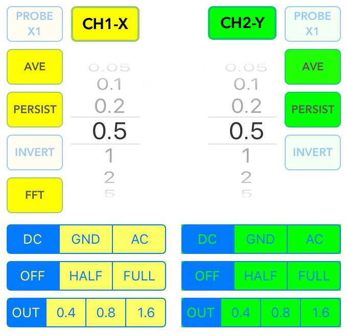 The main control is the input level picker. The values on the picker are modified by the Probe settings and will reflect the voltage ranges with the probe attenuation factor.
The channel name above the input picker turns the trace on or off. When in XY mode the channel name indicates its axis.
AVE averages a trace with a user set number of previous traces.
PERSIST show a user set number of past traces that fade with age.
INVERT inverts the trace including any DC offset.
FFT will select this channel as the signal source for the FFT.
The top segmented bar is the input coupling selector.
The middle segmented control is the auto-ranging feature. The system will keep the trace to no more than half or full scope display height by changing the input’s level picker.
The bottom segmented control is for rolling average noise reduction. The numbers represent the percentage of total samples that will be averaged.
Sampling Controls
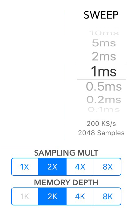 SWEEP is the main control here and determines the time/div value for the displayed trace. Below this control are labels indicating the memory storage rate and the memory size. The system always samples the input signal at 100MS/s but will skip storing samples in memory to achieve the sampling rate shown in the label. The memory depth divided by the sampling rate must always equal the total sweep time for the entire display.
Increasing the SAMPLING MULT setting will increase the sampling rate and the memory depth to achieve the same trace time but with more data points in the trace. The memory depth can be increased separately from the sampling multiplier setting which will produce more data than can be shown on the scope display. Panning the x-axis will display this additional data. Not all sampling multipliers are available for all sweep rates due to limitation in the clocking system. Unavailable setting are disabled.
Trigger Controls
Trigger source channel and slope edge controls are common 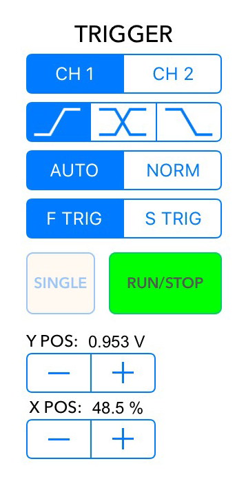 and self-explanatory except for the center selection for trigger slope which selects level only triggering.
The AUTO selection is for an auto baseline that ensures the trace will trigger even if an actual trigger was not detected. This ensures the trace is not static which can be confusing. In NORM mode AirScope will wait indefinitely for an actual trigger event before producing a trace.
F TRIG and S TRIG selects trigger detectors with different attributes. F TRIG is excellent at detecting fast moving signal changes, such as in a square wave. S TRIG is excellent at detecting trigger crossing points in very slowly changing signals.
RUN/STOP is the main operational control for the system.
SINGLE sets the system up for capturing and displaying a single trigger event.
The top Y POS stepper allows fine setting of the trigger voltage trip point. The X POS stepper allows fine setting of the trigger point in time relative to the display.
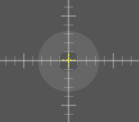 This donut shaped area in the scope display is the main control for setting the trigger point. Pressing the donut for a second activates the cursor which can then be dragged on the screen to the desired trigger point and released. This allow for fast and easy trigger setting.
Special Function Controls
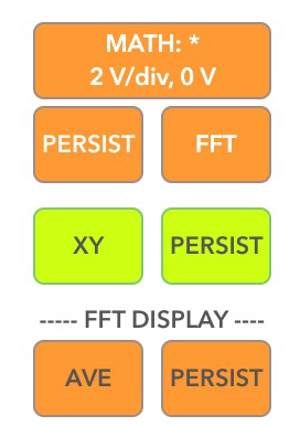 The MATH function allows channel 1 & 2 traces to be added, subtracted, multiplied or divided. Two user entry fields on the back panel allow for scaling and offsetting of the results. The button shows the math function in use as well as the scaling factor and the offset factor.
An FFT of the math result can be selected and persistence can also be applied.
The XY function allows amplitudes to be plotted against one another. There are separate positioning controls for each axis and persistence can be applied to the plot. The Circle graticule is provided to help identify phase shift issues in quadrature signals.
The FFT DISPLAY controls allow both trace averaging and persistence to be applied to the FFT trace regardless of which channel is using the FFT function.
 SNAPSHOT takes a screen capture and stores it in the camera roll section of the photos app. The timestamp in the bottom center of the panel is helpful in identifying image.
Indicators
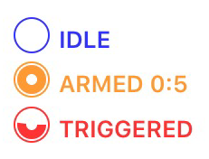 The Trigger Status Indicator provides feedback to the user about the current acquisition. The display is hidden until the trace repetition times are long enough to make the display meaningful. When the armed time is longer than 1s, the ARMED indicator will show the time in minutes : seconds since the trigger was armed. Helpful information when trigger events happen infrequently. The TRIGGERED indicator has a circular progress indicator to show the how long until the acquisition is complete. The IDLE indicator is shown when the AirScope is not actively acquiring a signal.
 The Battery Status indicator provides feedback in several ways. It indicates the battery charge level graphically with a bar that shortens and changes color as the battery is depleted. It also shows the actual battery pack voltage.
 The date and time display provides a means of identifying and differentiating snapshots since there is currently no way to name the image files.
BACK PANEL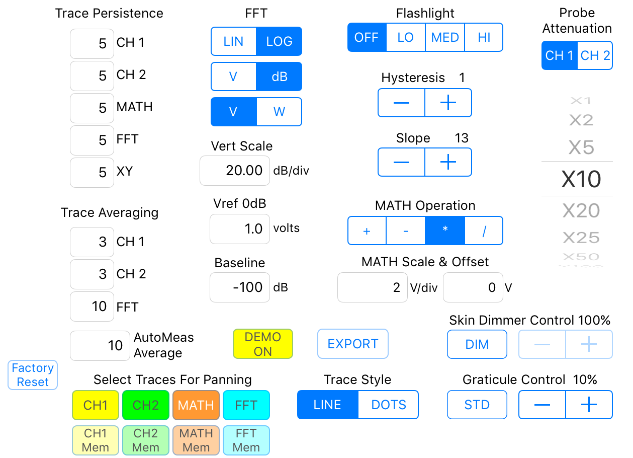
Persistence and Averaging Settings
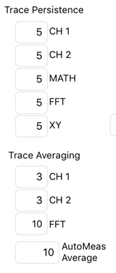
Each trace can have variable persistence applied to it. Variable persistence keeps a number of previous traces on the screen but progressively fades out the older traces. These settings determine how many traces will be kept.
Trace Averaging will average together the number of traces specified in the field. It takes very few traces to greatly reduce random noise on the trace. Measurements are calculated from of the trace data so they too will show the effects of the averaging.
The AutoMeas Averages field determines how many measurements will be averaged on the corner displays. The number here will affect measurement’s the settling time.
FFT Settings
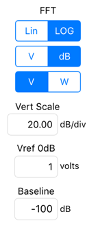 LIN / LOG – Selects the type of vertical scale for FFT.
V / dB – Selects units to be use in display. Volts can be displayed even if scale set to log. Only available in log.
V / W – Determines if dB conversion uses 10 or 20 as the divisor. Only available in log mode.
Vert Scale – User input field sets vertical scaling. It is dB/div in log mode and mV/div in lin mode.
Vref 0dB – User input field that sets the 0dB reference. Only available in log mode.
Baseline – The very bottom of the display represents the baseline for the FFT. The user input in this field sets the value of that position. Larger (less negative) numbers move the trace up.
Math Settings
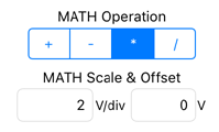 Select the math function from the segmented control. The math is performed using scaled data and it is usually necessary to adjust the scale and offset of the result to show the trace on screen at the desired size.
Probe Settings
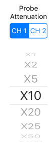
When the input’s PROBE button is active, the probe factor set here will be applied to the input level picker values and to all the measurement associated with the channel. The segmented control above the picker determines the channel the picker setting applies to.
Export Visible Traces

The Export function allows a .csv file containing all traces currently on screen, including trace memories, to be shared through the various resources available on the iPad (text, email, AirDrop, etc.). Time domain and FFT traces include X-axis labels for each data point.
The actual data size acquired by the AirScope is always a base-2 value (1024, 2048, 4096 or 8192) but in order for time domain data to display properly with the display scale, which is base-10, a portion of the beginning and end of the captured data is clipped off. When time domain data is exported that clipped off data are included in the file. The X-axis labels for the data before the first visible data point are negative. Including the full (base-2) data set allows the captured data to be compatible with other FFT analysis software.
Demo Mode
 The AirScope UI includes a Demo mode that supplies various waveforms that simulate the operation of the AirScope. Demo operation requires that the AirScope UI app NOT be connected to an actual AirScope, which is indicated by the red “NOT CONNECTED” status message on the connection button. With the AirScope UI in this mode and the Demo system enabled, simulation will commence by setting the Run/Stop button to run. Tapping the “NOT CONNECTED” button will cycle through a set of waveforms.
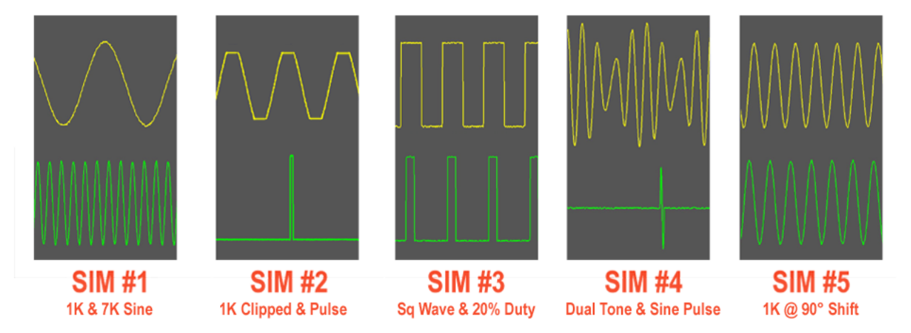
Connecting the AirScope UI app to an AirScope will suppress the Demo function, however it’s best to turn the Demo function off when it’s not needed. Nearly all functions of the AirScope UI work during demo operation. Only features that are specific to the hardware in the AirScope are non-functional. Those are: flashlight, noise reduction, trigger detector and LiveCal operation.
Skin Dimmer
 The rear panel contains a Skin Dimmer feature that allows the background intensity to be controlled. A button toggles the intensity between full “Bright” and a value set using the Skin Dimmer stepper control. Trace and graticule intensity are not affected by this control.
Graticule Controls
The button allows different graticule patterns to be cycled through. The associated stepper control sets the intensity of the graticule.
The graticule sits on top of the trace and can obscure portions of the trace. Reducing the graticule intensity allows these obscured portions to be seen.
Flashlight
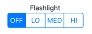 The flashlight at the back of the AirScope can be remotely controlled though this segmented bar. On the AirScope there is a push button that will cycle through these intensity settings. Any change made at the AirScope unit will be reflected here. In addition to its obvious purpose, the flashlight can be used to identify the currently connected AirScope if more than one exists.
This control is non-functional when running in Demo mode.
Trace Pan Control
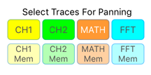
When one or more of these buttons is deselected, that button’s trace will be locked from panning. This can be used to superimpose one trace over another or to expose a memory trace that is covered by an active trace. A double tap on the scope display screen will unlock all the traces.
Trace Style
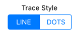 Determines if the traces are drawn with a continuous line or a series of dots that represent actual data points.
Factory Reset
All current user setting are automatically saved within the AirScope UI app to ensure that it opens in the last configuration. A Factory Reset button is provided to revert the configuration to the factory default settings. The reset procedure requires that after the Factory Reset button is pressed, the AirScope UI app is terminated. Terminating an app usually is done by double clicking the home button and then swiping up on representation of the particular app, but this could be different on your device. When the AirScope UI app is again launched all setting will revert to the initial factory ones.
Slope Detectors
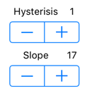 There are two types of slope detectors, these detectors ensure that the trigger happens on the correct edge of the waveform. The Hysteresis detector is used when the trigger is set to F TRIG for fast changing slopes, like square waves. The Hysteresis stepper adjusts the sensitivity of this detector. Setting the value higher requires more vertical distance between data points and can help prevent triggering on trace noise. If this is set too high for the particular signal, it may prevent triggering.
When the trigger is set to S TRIG, the Slope trigger detector is in use. This is for slow moving, low slope, signals. The stepper adjusts the number of samples the system uses to detect a trigger crossing. A higher value can improve triggering on shallow slopes but makes triggering at peaks unstable.
These controls have no effect when running in Demo mode.